Electrical Studies

Short-Circuit Current Studies conducted on electrical systems can serve various purposes, such as:

 

– Verifying the interrupting capacity of circuit breakers;

– Verifying the ability of circuit breakers to withstand the dynamic forces produced by maximum asymmetric short-circuit currents;

– Obtaining the subtransient and transient contributions of branches connected to the fault point, which serve as a basis for determining the protection device settings.

 

The main objective of these studies is, therefore, to determine the subtransient and transient contributions in order to define the appropriate settings for the protection devices.

 

In our studies, we use SKM’s PTW software, specifically the DAPPER module, which employs the technique of assembling the Nodal Admittance Matrix (Ybus) and subsequently inverts it to obtain the Impedance Matrix (Zbus).

 

Matrix Assembly Technique

 

Based on the one-line diagram and system data, the software generates the admittance matrix (Ybus). The Ybus matrix is square, with dimensions corresponding to the number of buses in the system. The characteristics of the Ybus matrix allow for its inversion, thus obtaining the impedance matrix (Zbus), which makes it possible to calculate the fault currents at the buses using Ohm’s Law.

 

Balanced Faults

 

Fault currents in a three-phase system can be either balanced across all three phases or unbalanced. Unbalanced faults involve one or two phases, but never all three. The symmetrical three-phase fault current (balanced fault) is often considered the maximum fault current at a bus. However, under certain system conditions, an unbalanced fault can result in a higher current than a three-phase fault.

For the calculations to be performed, Ohm’s First Law must be defined:

 

[E] = [Z]*[I]

 

Where:

 

E: Bus voltage matrix

 

Z: Bus impedance matrix; also known as the Zbus matrix

 

I: Bus nodal current matrix

 

The impedance Z in complex notation:

 

Z = R + jX

 

Where:

 

R: Resistance

 

jx: Reactance

 

 

Thevenin Equivalent Circuit

 

The short-circuit study formulates the node equations by applying Kirchhoff’s Current Law (KCL). To determine the fault current, the Thevenin equivalent (reduced) impedance is used for each fault point (node).

 

The short-circuit current is calculated by:

 

[I] = [E] / [Zth]

 

Asymmetrical Current

 

In the subtransient case, in addition to the symmetrical currents, the software also calculates the asymmetry factor based on the X/R ratio, and then determines the value of the asymmetrical current. These asymmetry factors are obtained from IEEE Std 241-1974, Table 61, page 241.

 

Unbalanced Faults

 

To calculate unbalanced fault currents, the FORTESCUE technique is used, i.e., symmetrical components, which decomposes the unbalanced system into three sequence networks: positive sequence, negative sequence, and zero sequence. This allows for the individual application of phasor theory to each sequence network, after which the results are converted back to phase values.

 

For single line-to-ground short-circuit currents, the positive, negative, and zero sequence networks are in phase, i.e., the current values are equal:

 

Ia = 3Ia0 (This means that the sequence networks are connected in series, as they share the same current).

 

Va = Va0 + Va1 + Va2 = 0

 

Va0 = -Zo*Iao

 

Va1 = E – Z1*Ia1

 

Va0 = -Z2*Ia2

 

Va = E – Z1*Ia1 – Zo*Iao – Z2*Ia2 = 0

 

Since, Iao = Ia1 = Ia2:

 

E = Z1*Ia1 + Z2*Ia1 + Zo*Ia1

 

E = (Z1 + Z2 + Zo)*Ia1

 

Ia1 = E/(Z1 + Z2 + Zo)

 

Ia2 = Iao = E/(Z1 + Z2 + Zo)

 

In the faulted phase (phase “A”), the current will be:

 

Ia = 3Ia1

 

Ia = 3E/(Z1 + Z2 + Zo)

 

Thus, the magnitude of the single line-to-ground fault current is given by:

 

Icc1f = 3E/(Z1 + Z2 + Zo)

 

Taking into account the neutral grounding method, the above formula can be modified as follows:

 

Icc1f = 3E(Z1 + Z2 + Zo + 3Zn)

 

Asymmetrical Current

 

In the subtransient case, in addition to symmetrical currents, the software also calculates the asymmetry factor based on the X/R ratio, and subsequently determines the value of the asymmetrical current. These asymmetry factors are obtained from IEEE Std 241-1974, Table 61, page 241.

 

How to Calculate a Short Circuit?

 

What Are the Formulas for Calculating Short-Circuit Current?

 

Below is an example of a short-circuit calculation, highlighting the formulas for calculating both symmetrical and asymmetrical three-phase short-circuit currents at each point.

 

1. Basic Theory on Short-Circuit Calculations in Industrial Electrical Installations

 

           Short-circuit currents primarily depend on the impedances between the source and the point where the fault occurs (such as busbars, cables, and machine terminals). Certain types of loads, such as motors, can also contribute to higher short-circuit levels. However, their influence is generally much lower than that of the utility supply. In this article, the influence of motors on short-circuit levels will not be addressed. Thus, the short-circuit will be considered solely as a function of the impedances between the utility supply and the fault location.

 

          According to Mamede Filho (2010), points far from the generation source are heavily influenced by the impedance of transmission lines, since their impedance is much greater than that of generators. Therefore, the short-circuit current consists of two basic components, graphically represented in Figure 1.1:

 

– Symmetrical Component: As the name implies, this is the symmetrical portion of the current, which predominates a few cycles after the short circuit occurs.

– DC Component: This is the unidirectional component whose value decays over time, due to the inability of magnetic flux in the system to change instantaneously.

 

Figure 1.1 – Current waveform during a short circuit (Source: SKM, 2006a, 2006b)

 

2. Simplified Methodology for Calculating Three-Phase Short-Circuit Current

 

          The most commonly used method for calculating short-circuit current in practice is the per-unit system, also known as the “pu” method. The value of an electrical quantity (voltage, current, power, impedance, etc.) is defined as the ratio between its actual value and a predefined base value.

 

          The main advantage of this method lies in the fact that power systems typically operate at different voltage levels due to the presence of transformers. By using per-unit values, transformers can be represented simply by their impedance, as if their turns ratio were 1:1, thus simplifying the calculations.

 

To illustrate the analyses in this study, all calculations will be based on the theoretical system presented in the diagram in Figure 2.1.

 

Figure 2.1 – One-line diagram of the theoretical system to be studied

 

2.1 Definition of Bases

 

Initially, the bases to be used for the per-unit calculations must be chosen. In general, a typical value of 100 MVA is used for the base power (Pb).

 

P_b = 100MVA (2.1)

 

For the base voltage (Vb), it is common to use the highest voltage level in the system under study. In our case, we will work with a system at 13.800 V:

 

V_b = 13.800 V (2.2)

 

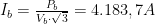
From these values, we can calculate the base current (Ib):

 

 

2.2 Utility Impedance and Short-Circuit Levels

 

The impedance may be provided by the utility directly in per-unit (pu), or, if given in Amperes, it must be converted to a per-unit value.

 

Z_1(pu)utility =     I_b / I_{sc3øsymutility} (2.4)

 

Where:

 

I_{sc3øsymutility} – Symmetrical Three-Phase Short-Circuit Current at the utility’s delivery point.

 

I_b – Base Current.

 

Z_1(pu)utility – Positive Sequence Impedance in per-unit at the utility’s delivery point.

 

2.3 Transformer Impedance

 

Z_1(pu)tr =Z_% ^. P_b / P_t (2.5)

 

R_1(pu)tr = R_% ^. P_b / P_t (2.6)

 

X_1(pu)tr = ( Z_(pu)² – R_(pu)²) ^½  (2.7)

 

             Where:

 

Z_1(pu)tr,  R_1(pu)tr,  X_1(pu)tr – Positive Sequence Impedance, Resistance, and Inductive Reactance of the Transformer

 

Z_% – Transformer Percent Impedance (Nameplate Data)

 

P_t – Transformer Power (in VA)

 

P_b – Base Power (100 MVA)

 

 

2.4 Cable impedance

 

R_1(pu)cable = ((R_{per meter}  x  P_b  )/V²  ) x dist / ncpp (2.8)

 

X_1(pu)cable = ((X_{per meter}  x  P_b  )/V²  ) x dist / ncpp  (2.9)

 

Z_1(pu)cable =  ( R_(pu) ² + X_(pu)² ) ^½  (2.10)

 

Where:

 

R_1(pu)cable, X_1(pu)cable, Z_1(pu)cable –Resistance, inductive reactance, and positive sequence impedance of the cable.

 

R_{per meter} e X_{per meter} – Resistance and inductive reactance per meter (manufacturer’s data).

 

P_b – Base Power (100MVA)

 

V – Nominal voltage of the cable circuit (in volts).

 

Dist – Distance (in meters).

 

ncpp – Number of cables per phase.

 

2.5 – Calculation of Three-Phase Short-Circuit Currents

 

I_sc3øsym = I_b / Z_(pu) (2.11)

 

 

Where:

 

I_sc3øsym – Symmetrical Short-Circuit Current.

 

I_b – Base Current.

 

Z_(pu) – Equivalent Impedance at each point in per-unit.

 

I_sc3øasym – Asymmetrical Short-Circuit Current.

 

e – Euler’s number (2,71828)

 

π – “pi” (3,14159)

 

X/R – Ratio between the positive sequence inductive reactance and positive sequence resistance at the point where the asymmetrical short-circuit current is to be calculated.

 

 

3. Example of Three-Phase Short-Circuit Calculation

 

To illustrate the equations presented in Section 2 and to validate the effectiveness of the calculations performed in simulations using PTW software version 6.5.2.7, we present the short-circuit level calculations made for the system exemplified in Figure 2, also considering the data from Tables 3.1 to 3.4.

 

Table 3.1 – Utility Data

 

Short-Circuit Current Level at the Delivery Point (A)	X/R Ratio
5.000	8

 

 

Table 3.2 – Medium Voltage Cable Impedance

 

Cable	Positive Sequence Resistance per meter (Ω/km)	Positive Sequence Inductive Reactance per meter (Ω/km)
50mm2 (8,7/15kV)	0,4938	0,1551
35mm2 (8,7/15kV)	0,6684	0,1651
25mm2 (8,7/15kV)	0,9272	0,1726

 

Source: Ficap Catalog, Fipex 8.7/15 kV cables, single-core, installed in trefoil configuration

 

Table 3.3 – Low Voltage Cable Impedance

 

Cable	Positive Sequence Resistance per meter (Ω/km)	Positive Sequence Inductive Reactance per meter (Ω/km)
25mm2 (0,6/1kV)	0,9362	0,1150
240mm2 (0,6/1kV)	0,1009	0,0980
185mm2 (0,6/1kV)	0,1303	0,0980

 

Source: Ficap Catalog, Fipex 0.6/1 kV cables, single-core, installed in trefoil configuration

 

Table 3.4 – Transformer Data

 

Transformer	Power (kVA)	Voltage (V)	Percent Impedance (Z%)	Percent Resistance (R%)
TR01	2.000	13.800 – 440/254	6,5%	1,1%
TR02	112,5	13.800 – 220/127	4,49%	2,56%

 

 

3.1 Calculation of System Impedances in Per Unit (pu)

 

Considering our bases as Pb = 100 MVA and Vb = 13.800 V, and applying Equation 2.4 to the utility data (Table 3.1), the results are obtained as shown in Table 3.5:

 

Table 3.5 – Utility Impedance Values in per unit (pu)

 

Positive Sequence Resistance in per unit (pu)	Positive Sequence Inductive Reactance in per unit (pu)
0.103785	0.830278

 

By applying Equation 2.8 to the cables, the results are obtained as shown in Table 3.6:

 

Table 3.6 – Cable Impedance Values in per unit (pu)

 

Cables	Conductor Size / Insulation	Distance	Cables per phase	Positive Sequence Resistance in per unit (pu)	Positive Sequence Inductive Reactance in per unit (pu)
General MV Cable	50mm2(8,7/15kV)	20 m	1	0.0052	0.0016
MV Cable TR01	35mm2(8,7/15kV)	20 m	1	0.0070	0.0017
MV Cable TR02	25mm2(8,7/15kV)	20 m	1	0.0097	0.0018
LV Cable TR01	240mm2(0,6/1kV)	20 m	8	0.1303	0.1265
LV Cable TR02	185mm2(0,6/1kV)	20 m	1	5.3843	4.0496

 

By applying Equations 2.5, 2.6, and 2.7 to the transformers, we obtain the results shown in Table 3.7:

 

Table 3.7 – Transformer Impedance Values in per unit (pu)

 

Transformer	Power (kVA)	Voltage (V)	Resistance (pu)	Inductive Reactance (pu)
TR01	2.000	13.800 – 440/254	0.5500	3.2031
TR02	112,5	13.800 – 220/127	22.7556	32.8000

 

 

3.2 Calculation of Equivalent Impedances in per unit (pu) for Various Points in the System

 

The equivalent impedance at the General Substation (ST-General) is given by the vector sum of the utility and the General MV Cable impedances:

 

Zeq_ST-General = Zutility + Z_{MV General Cable} = 0,103785 + j0,830278 + 0,0052 + j0,0016

 

Zeq_ST-General = 0,108985 + j0,831878 pu

 

Zeq_ST-General = 0,8390 pu (angle =  82,53^o)

 

By applying Equations 2.11 and 2.12, we obtain the short-circuit values for the General Substation (ST-General):

 

I_{sc3øsym ST-General} = 4.183,70 / 0,8390 = 4.986A

 

I_{sc3øasym ST-General} = 6.834A 

 

The equivalent impedance at the primary of TR-01 (ST-TR01) is given by the vector sum of the impedances of the utility, the General MV Cable, and the MV Cable for TR01:

 

Zeq_ST-TR01 = Z_utility + Z_{MV General cable} + Z_{MV cable TR01} = 0,103785 + j0,830278 + 0,0052 + j0,0016 + 0,0070 + j0,0017

 

Zeq_ST-TR01 = 0,115985 + j0,833578 pu

 

Zeq_ST-TR01 = 0,8417 pu (angle =  82,07^o)

 

By applying Equations 2.11 and 2.12, we obtain the short-circuit values for Substation TR-01 (ST TR-01):

 

I_{sc3øsym ST-TR01} = 4.183,70 / 0,8417 = 4.971 A

 

I_{sc3øasym ST-TR01} = 6.732 A 

 

Performing the calculations for the other points of the system in a similar manner, we obtain the results shown in Table 3.8, which presents the values of symmetrical and asymmetrical three-phase short-circuit currents. It should be noted that, for points located at low voltage, the levels have already been calculated for the nominal voltage of each panel; that is, the results obtained through Equations 2.11 and 2.12 have already been multiplied by the transformation ratio.

 

Table 3.8 – Calculated Three-Phase Short-Circuit Levels

 

Point	Voltage (V)	Zeq (pu)	Isc3øsym(A)	X/R Ratio:	Isc3øasym (A)
Consumer Entry	13800	0.8367	5000	8	6914
ST General	13800	0.8390	4986	7.63	6834
ST TR01	13800	0.8417	4971	7.19	6732
ST TR02	13800	0.8421	4968	7.02	6698
PGLV-01	440	4.2388	30956	5.23	39173
PGLV-02	220	47.1018	5572	1.33	5621
CCM01	440	4.8518	27045	3.54	31304
CCM02	440	5.4926	23890	2.81	26329
CCM03	440	6.1524	21327	2.41	22843
CCM04	440	6.8259	19223	2.15	20228
QLF01	220	79.2611	3311	0.63	3311
QLF02	220	115.6912	2268	0.45	2268
QLF03	220	153.3784	1711	0.36	1711

 

 

References

 

1. Mamede Filho, Instalações Elétricas Industriais, Rio de Janeiro, LTC, 2010

 

SKM Systems Analysis, Inc. Power Tools for Windows – A Fault Reference Manual – Electrical Engineering Analysis Software for Windows, Manhattan, USA, SKM, 2006a.

 

SKM Systems Analysis, Inc. Power Tools for Windows – A Fault Reference Manual – Electrical Engineering Analysis Software for Windows, Manhattan, USA, SKM, 2006b.

 

 Arc Flash Study, ATPV Study and Incident Energy Calculation

The Arc Flash Study estimates the exposure to incident energy originating from arc flash sources. To understand the purpose of the arc flash study, it is important to distinguish between traditional faults and arc faults. A bolted three-phase, phase-to-phase, or phase-to-ground fault creates high currents that flow through the power system. Traditional fault studies are used to size equipment capable of withstanding and interrupting these short-circuit currents. Arc fault currents occur when electrical current passes through the air between two conductive materials, producing extremely high temperatures. These high temperatures can cause fatal burns even at several meters from the arc source. The arc also results in the ejection of molten material in the surrounding area, posing an additional hazard. Arc fault current is lower than that of a traditional fault, as the arc itself acts as a resistive path between conductors.

The study below was developed in accordance with NFPA 70E and IEEE 1584 standards, determining safe working distances and the amount of incident energy to which a worker may be exposed when working near electrical equipment. Burns caused by arc flashes account for a significant portion of electrical work-related accidents.

The study combines short-circuit calculations, empirical equations, and protection device operating times to estimate the incident energy, Personal Protective Equipment (PPE) levels, and approach boundaries.

 

Basic Concepts on Arc Flash Study, ATPV Assessment and Incident Energy Calculation

The Arc Flash Study is meticulously conducted to evaluate the incident energy generated by arc flash events.

The study includes a set of essential parameters, described below:

– Arc Flash

It is the source of energy released between two conductors or between a conductor and ground.
This energy is generated by an electrical current that travels through the arc path.

– Normalized Incident Energy

At the moment of a fault, energy is released into the surrounding space due to the arc, typically lasting about 200 milliseconds, and calculated for a human body positioned 600 mm (24 inches) from the arc.

Incident energy is a function of voltage, short-circuit current, and clearing time of protective devices. It is inversely proportional to the working distance.

 

– Incident Energy

This is the calculated energy, derived from the normalized incident energy, that reaches a worker’s skin or protective clothing.

– ATPV (Arch Thermal Performance Value) as defined by ASTM F1959-06.

Thermal performance of a material, referring to the amount of incident energy the material can withstand before the wearer suffers second-degree burns. Higher ATPV values indicate better protection against arc flash hazards.

– Flash Protection Boundary or AFB – Arc Flash Boundary

This is the minimum safe distance from an arc source at which a person may be exposed to 1.2 cal/cm² (5 J/cm²) of incident energy, enough to cause second-degree burns on unprotected skin.

– Risk Zone (NR10)

The zone around an energized conductive part, not physically segregated, and accessible even accidentally. Its dimensions are defined by the voltage level, and only authorized personnel with proper tools and techniques may approach it.

– Controlled Zone (NR10)

An area around energized conductive parts, not physically segregated but accessible, with defined dimensions according to the voltage level, where only authorized professionals may enter.

Common Causes of Arc Flash Incidents:

– Loose or Poor Connections (e.g., improperly torqued terminals)
– Insulation Degradation (due to overvoltage, overload, etc)
– Defective Components/Equipment (undetected faults that manifest during the operational life)
– Undersized or Poorly Designed Installations
– Accidental Contact (e.g., tools, metal parts, or foreign objects creating a fault path)

 

Calculation Methodology

 

– Arc Current

To determine arc fault currents, we follow the procedure described in IEEE 1584 and Annex D.8.2 of NFPA 70E:

The calculation is based on the short-circuit current, which is converted to an equivalent arc current.
The method for calculating short-circuit currents proposed in IEEE 1584 is detailed in IEEE Std. 141 – 1993. The software PTW (Power Tools for Windows) utilizes results obtained through the Comprehensive method in the DAPPER module, which is fully applicable for determining short-circuit currents. For the fault condition analysis, data sets provided by the ONS (Brazilian National Electric System Operator) were used, specifically: “ONS * SISTEMA INTERLIGADO * CONF JUNHO/2013 VERSÃO 13/08/2013 * BR1306A.ANA”. The corresponding short-circuit levels are presented in the attached study and in the tables provided in section 1.5.

 

Low Voltage Systems (up to 1 kV):

 

 

– Incident Energy Calculation:

 

Where:

Ia = Arc Current [kA]
K = – 0.153for open-air configuration
K = – 0.097 for enclosed configuration
Ibf = Three-phase symmetrical fault current RMS [kA]
V = System voltage [kV]
G = Gap between conductors [mm]

 

For system voltages between 1 kV and 15 kV, there is no distinction between open-air and enclosed configurations. Therefore, the following equation should be applied:

 

 

– Normalized Incident Energy Calculation

The normalized incident energy is calculated as presented in item 5.3 of the standard:

 

Where:

 

 

NE = Normalized Energy [J/cm²]
K1 = – 0.792 for open-air configuration
K1 = – 0.555 for enclosed configuration
K2 = 0 for isolated or resistance-grounded systems
K2 = – 0.133 for solidly grounded systems
G = Gap between conductors [mm]

Where:

 

 

 

E = Incident Energy
Cf = 1 for voltages <1 KV
Cf = 1,5 for voltages ≥ 1KV
NE = Normalized Energy [J/cm²]
t = Protection device operating time
D = Working distance [mm] (as per NFPA 70E Table D.7.3).
X = Distance exponent (as per NFPA 70E Table D.7.2).

The following tables are extracted from NFPA 70E Annex D.

 

Table D.7.2

 

 

Table D.7.3

 

 

The typical working distance is the sum of the distance between the worker and the front of the equipment, plus the distance between the front and the source of the arc origin, located inside the equipment.

 

– Response Time of Protection Equipment

 

Using the time obtained from the selectivity study of the protection relays, and the relay processing time provided by the manufacturer—which is equivalent to 1/4 of a cycle (0.004 s) for relays without arc protection, and 1/16 of a cycle (0.001 s) for relays with arc protection, we add to these times the corresponding actuation time of the protection device, where each device has an inherent time that varies from manufacturer to manufacturer.

The following table, extracted from the IEEE 1584 Standard, provides typical actuation times for the isolation system:

 

 

Based on safety considerations, the Opening Times of the Devices used in this study were:

Low Voltage: 3 cycles (0,050 s)
Medium Voltage: 8 cycles (0,080 s)

 

– Phase-to-Phase Distance (GAP)

Through standardized tests, a series of reference values were obtained, focusing on the working distance and the protection device operating time. According to these values, we can determine the recommended GAP between phases for the calculation, as shown in the following table extracted from the IEEE Standard – 1584:

 

 

In this study, the distances used were based on the construction drawings of the panels and cubicles:

Medium Voltage Cubicles: 90 mm;
CDC: 20 mm;
CCM: 25 mm (according to the NFPA recommendation, considering that the actual distance is greater).

 

– Safe Approach Distance Against Arc Flash (IEEE 1584)

 

Limit distance from the energy source (arc) at which the worker is still exposed to second-degree burns due to the heat generated by the arc, equivalent to 1.2 cal/cm² or 5.0 J/cm². To determine the safe approach distance, the following equation should be applied:

 

 

AD = Approach distance from the arc point (mm)
Cf = 1 for voltages <1 KV
Cf = 1,5 for voltages ≥ 1KV
NE = Normalized Energy [J/cm²]
IE = Incident energy [J/cm²] at the protection distance
t = Protection device operating time
X = Distance exponent (according to table D.7.2 of NFPA 70E)

 

Table of PPE Protection Levels Based on Calculated Incident Energy (NR10)